Table of Content
1. Introduction
The Malta Shelf model ROSARIO-II hydrodynamical is an eddy-resolving primitive equation sigma level shelf-scale numerical model. It is run at two spatial resolutions 1/64°x1/64° and 1/96°x1/96° with
a grid ratio of 1:2 with respect to the regional model in both cases. The model includes full thermohaline dynamics and adopts a turbulence scheme for the vertical mixing coefficients on the basis of the Princeton Ocean Model. It is implemented within the study area (from 13.80°E to
14.94°E and from 35.42°N to 37.21°N) with 115 grid points in latitude and 74 in longitude for the lower resolution and grid points in latitude and longitude for a higher resolution version. The model has three open boundaries (on the West, South and East).
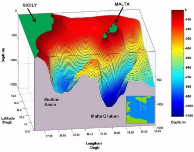
In the vertical it has 20 sigma layers (bottom following) with logarithmic distribution near the surface. The model bathymetry used is that from the U.S. Navy bathymetric database by interpolation of the data (mapped on a 1/60x1/60 degree in latitude and longitude) into the model grid.
2. Model Characteristics and Setup
The numerical code used is based on an application of the Princeton Ocean Model, POM (Blumberg and Mellor, 1987). POM is a primitive equation, stratified and nonlinear numerical ocean model which utilises the Boussinesq approximation and hydrostatic equilibrium. It uses the free surface, potential temperature and salinity, the three orthogonal components of velocity, the turbulence kinetic energy and the turbulence macroscale as the prognostic variables. The model features include a split mode time step and a sigma-coordinate transformation for the vertical grid.
The bottom following sigma layers allow the model to represent accurately regions of high topographic variability. The horizontal grid uses curvilinear orthogonal coordinates and an “Arakawa C” differencing scheme. The Mellor and Yamada (1982) turbulence closure scheme is used to calculate the coefficients of vertical mixing of momentum, the vertical eddy viscosity and the eddy diffusivity of heat and salt. Density is calculated by an adaptation of the UNESCO equation of state revised by Mellor (1991).
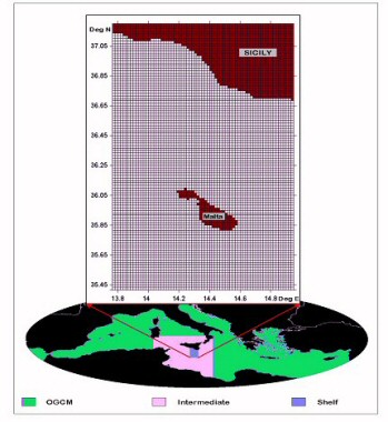
The details of the model implementation are described in Table 1. The nesting of temperature, salinity and velocities (total and barotropic), is necessary in order to transfer values of variables from the Sicilian Channel Regional Model (SCRM) coarsely spaced grid to the shelf scale higher resolution grid at the location of the open lateral boundaries. The nesting between the coarse and high resolution models is shown in Fig. 3. The SCRM daily mean fields are interpolated in space over the higher resolution grid and in time at each model integration (4 sec). The grid point data are filled by bilinear interpolation from the surrounding values. The specification of boundary data are calculated by interpolating linearly in time the values derived from the daily mean SCRM fields by an off-line, one-way nesting procedure similar to that adopted in MFSPP. The external normal velocities are imposed at each time step following the equation (Zavatarelli et al., 1999):
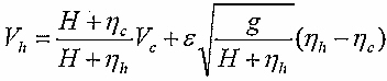
where Vh is the vertically integrated velocity on the model boundary, H is the bottom depth, h is the free surface elevation and VC is the vertical integral of the velocity at the boundary prescribed from the coarse model. The total velocities normal to the boundary are directly specified from the coarse
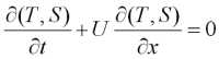
model. The mass transport at each respective open boundary is constrained to be equal to that prescribed from the SCRM. The tangential component velocities at the boundaries are set equal to zero. The free surface elevation is not nested (zero gradient boundary condition), while an upstream advection for temperature and salinity is used. In cases of outflow through the open boundaries, temperature and salinity are prescribed from the SCRM.
The reading and updating of the lateral boundary conditions from the regional model is done through the temporal interpolation of SCRM daily fields that are organised in weekly files. This is automated through a series of script files and dedicated codes that will eventually serve for the successive phases of the project when we will be preparing forecasts during the pre-TOP and TOP periods.
The model adopts an asynchronous air-sea coupling scheme consisting of a well-tuned set of bulk formulae to compute the momentum, heat and freshwater fluxes at the air-sea interface from the SKIRON forecast atmospheric data (at 1 hour intervals and 0.1deg Spatial Resolution, and the interactive updating of the heat flux components on the basis of the ocean surface temperature simulated within the model.
| Table 1 Malta Shelf Model Summary Description in forecast mode |
Model name : ROSARIO-II Malta Shelf Model based on the Princeton Ocean Model.
Forecast duration: 4 days (Thursday, Friday, Saturday and Sunday)
Geographic area coordinates : 13.80°E-14.94°E; 35.42°N-37.21°N
Grid, horizontal resolution : orthogonal grid at 1/64° (at 1.5 Km) or 1/96° (at 1 Km) with 20 sigma layers in the vertical direction grid nesting ratio with regional model = 2:1
Projection: Mercator
Topographic data used : DBDB1 bi-linearly interpolated into the model grid.
Model outputs : Temperature, Salinity, Barotropic velocity, Total velocity, Total heat flux, Evaporation – Precipitation,
Time sampling: 3 hours
Initialisation: Downscaling from MFSTEP-OGCM to the SCRM and to ROSARIO-II. The velocity, temperature and salinity fields from the SCRM simulation are mapped into the model grid using a bilinear interpolation scheme.
Internal Time Step: 90 seconds
External Time Step: 3 seconds
Horizontal Kinematic Viscosity: constant (5 m 2s -1)
Advaction of tracers: Smolarkiewicz upstream scheme with anti-diffusive velocities
Lateral Boundary Conditions : One-way nesting with the MFSTEP Sicilian Channel Regional Model (SCRM)
- Elevation: zero-gradient
- Barotropic normal velocities:
- Total normal velocities: V h=V cwith constraint of constant mass transport applied at each lateral boundary imposed every internal time step
- Tangential total & barotropic velocities set equal to course model values
- Temperature and Salinity: upstream advection
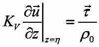
Surface Boundary Conditions : One way asynchronous coupling with the SKIRON atmospheric forecast fields at 1 hour intervals and 0.1 deg. spatial resolution.
where r 0 = density; t = wind stress calculated from the surface winds at 10m using the
Hellerman and Rosentein (1983) formula.
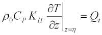
where C P = specific heat capacity at constant pressure; Q t = surface total heat flux.
where the evaporation rate E is expressed as the ratio Q e/L e ; and precipitation P is obtained from monthly climatological values by Jaegar’s and Legates. |
The momentum flux is calculated using the Hellerman and Rosentein (1983) formula. The surface boundary condition for heat utilises the updated sea surface temperature and salinity and therefore depends directly upon the state of the ocean. The total heat flux (Q t) consists of the short wave flux (Q sol) minus the net long-wave radiation (Q b) and the latent (Q e) and sensible (Q h) heat fluxes:
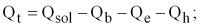
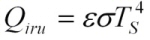
QB = Qiru – Qird, where Qiru is the upward IR flux emitted by the ocean and Qird is the downward atmospheric IR reaching the ocean. The long wave radiation flux (Qb) is calculated using the Bignami formula (Bignami et al., 1995) . The latent (Qe) and sensible (Qh) heat fluxes are given by the bulk aerodynamic formulae using the Kondo scheme for the turbulent exchange coefficients (Kondo, 1975).
The density of moist air  is computed by the model as a function of air temperature and relative humidity. The latent heat of vaporisation Lv is calculated as a function of the sea surface temperature (Gill, 1982). The turbulent exchange coefficients CE and Cv are estimated in terms of the air-sea temperature difference and the wind speed by an atmospheric stability index according to the Kondo parametrisation (Kondo, 1975). is computed by the model as a function of air temperature and relative humidity. The latent heat of vaporisation Lv is calculated as a function of the sea surface temperature (Gill, 1982). The turbulent exchange coefficients CE and Cv are estimated in terms of the air-sea temperature difference and the wind speed by an atmospheric stability index according to the Kondo parametrisation (Kondo, 1975).
| Q s and Q ird are provided directly from the atmospheric model and |
 |
For the salinity flux we consider:
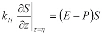
where the evaporation rate E is expressed as the ratio Qe/Le while precipitation P is obtained from the SKIRON forecast. |